Motivation & Objective

In the Real Estate (RE) industry, pricing is generally done by experts, considering the asset's features, the current market conditions, and sometimes the financial and time constraints relative to the RE project. These constraints can be bank loan repayment debts, and/or deadlines to entirely sell a property (e.g. all units of a building). This project aims at getting rid of the biases introduced by realtors and at fully taking into account the financial and time constraints, as well as the current inventory in the pricing process. It also aims at making pricing dynamic: reeavaluating assets prices under current inventory and satisfaction of the financial constraints.

The project's scope extends from sales and listings data scraping, to devising the pricing algorithm and testing it in a simulation environment.

Approach

There are multiple building blocks to this project:

• Data Scraping: The data required by the ML and optimization algorithms can be scraped on the main real estate market places. Information about both current listings and previous sales can be found in a such way.
• Market Value and Time-on-Market ML models: Using past sales data, it is easy to build two ML models assigning to each asset a market value and a predicted absorption time: the time an asset takes to sell once it is listed at a certain price. The Market Value model is Gradient Boosted Trees that are fitted on previous sale prices. Making the assumption that this model gives a true market value, it is possible to estimate from the model's error, an overpricing coefficient for every past sale. This overpricing coefficient is used as a predictor to derive the absorption time of RE assets.
• Dynamic Pricing Algorithm: This algorithm adapts RE assets prices in time, in order to satisfy financial and time constraints (revenues and # of sales targets in time). Monitoring actual sale and revenue rates and comparing them to the expected ones, RE assets' prices can be adapted to satisfy financial and time constraints. The starting price can be informed by the Market Value model and the algorithm's parameters can be informed by the time-on-market model.
• Simulation: It is possible to simulate demand (on the whole market, on the whole inventory and on unique assets) using past sales data, by making a few assumptions. Using the overpricing distribution of past sales it is possible to make the demand dependent on the assets' prices.

Results

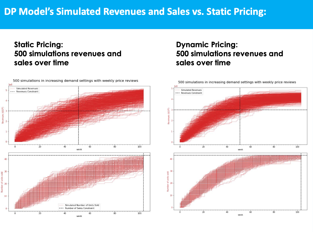
Putting everything together, given information on a building and its units layout, it is possible to build an algorithm that prices monthly every building's unit. The simulation environment allows to compare a static pricing strategy to the Dynamic Pricing algorithm.

More thorough explanation and visualizations can be found in the summary slides (cf. link at the top of the page).

References

• Dynamic Pricing Algorithm: Besbes, Omar, and Costis Maglaras. “Dynamic Pricing with Financial Milestones: Feedback-Form Policies.” Management Science 58, no. 9 (2012): 1715–31.